NoSQL and NewSQL
1. Context
This session presents newer types of data management systems, namely NoSQL systems and NewSQL database systems, which are frequently associated with big data settings. Big data may be characterized by 5 Vs [GBR15], namely large Volume, high Velocity (speed of data production and processing), diverse Variety (data from different sources may be heterogeneous; structured, semi-structured, or unstructured), unknown Veracity (raising concerns related to data quality and trust), potential Value (e.g., as basis for business intelligence or analytics). NoSQL and NewSQL address those Vs differently: Both promise scalability, addressing Volume and Velocity. NoSQL systems come with flexible data models, addressing Variety. NewSQL database systems perform ACID transactions, addressing Veracity. Value is up for discussion.
This text is meant to introduce you to general concepts that are relevant in videos in Learnweb (and beyond) and to point you to current research.
1.1. Prerequisites
- Explain notions of database system and ACID transaction (very brief recap below).
1.2. Learning Objectives
- Apply Amdahl’s and Gustafson’s laws to reason about speedup under parallelization.
- Explain the notions of consistency in database contexts and of eventual consistency under quorum replication.
- Explain the intuition of the CAP Theorem and discuss its implications.
- Explain objectives and characteristics of “NoSQL” and “NewSQL” systems in view of big data scenarios.
2. Background
2.1. Scalability
A system is scalable if it benefits “appropriately” from an increase in compute resources. E.g., if resources are increased by a factor of 2, throughput should be about twice as high for a system that scales linearly.
As previously mentioned in the context of query optimization, scaling of computers comes in two major variants: scaling up (also called scaling vertically) and scaling out (also called scaling horizontally or sharding). When scaling up (see Figure 1), we improve resources of a single machine (e.g., we add more RAM, more/faster CPU cores), while scaling out (see Figure 2) means to add more machines and to distribute the load over those machines subsequently, for example with horizontal fragmentation.
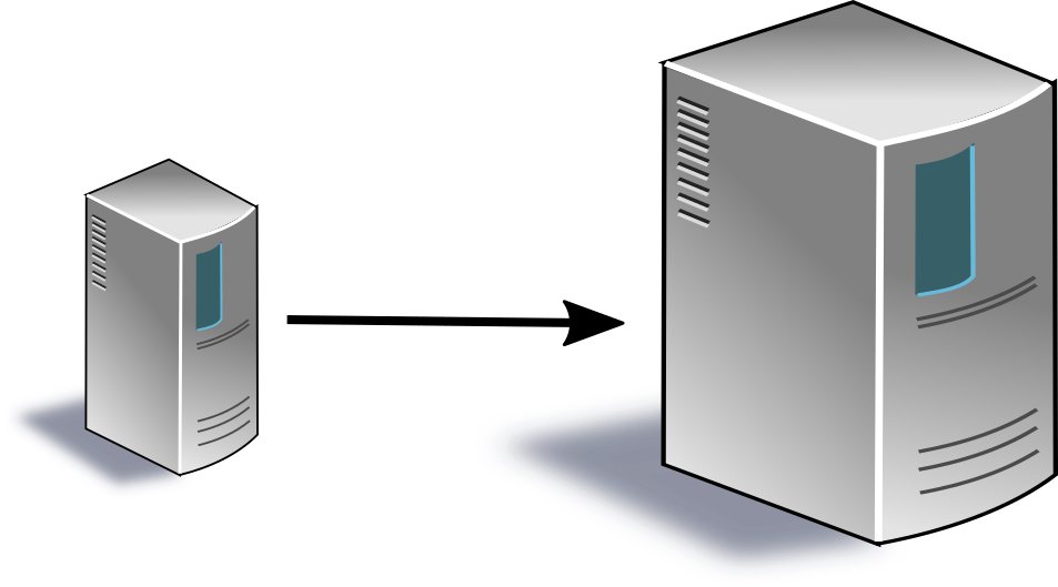
Figure 1: Scaling up improves the performance of a single machine.
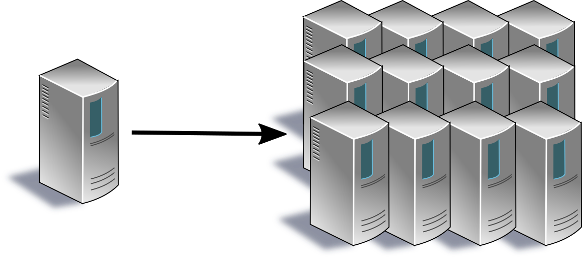
Figure 2: Scaling out distributes load over a fleet of systems.
Scaling out is not limited by physical restrictions of any single machine and is the usual approach in the context of big data. Indeed, [CP14] characterizes big data as being “large enough to benefit significantly from parallel computation across a fleet of systems, where the efficient orchestration of the computation is itself a considerable challenge.”
2.2. Limits to Scalability
Amdahl’s law [Amd67] provides an upper bound for the speedup that can be gained by parallelizing computations which (also) include a non-parallelizable portion. More specifically, if some computation is parallelized to \(N\) machines and involves a serial fraction \(s\) that cannot be parallelized, the speedup is limited as follows (the time needed for \(s\) does not change, while the remainder, \(1-s\), is scaled down linearly with \(N\)):
\[ Speedup = \frac{1}{s + \frac{1-s}{N}} \]
In the following interactive GeoGebra graphic you see a plot of this speedup (with \(N\) on the x-axis; the plot also includes a limit for that speedup and an alternative speedup according to Gustafson’s law, both to be explained subsequently).
E.g., consider a computation of which 90% are parallelizable (i.e., \(s=0.1\)), to be executed on \(N=10\) machines. You might guess the speedup to be close to 90% of 10, while you find only 5.3 given the above equation. For \(N=100\) and \(N=1000\) we obtain 9.2 and 9.9, respectively. Indeed, note that for \(N\) approaching infinity the fraction \(\frac{1-s}{N}\) disappears; for \(s=0.1\), the speedup is limited by 10. Suppose we scale the computation (e.g., in a cloud infrastructure or on premise). When scaling from 10 to 100 machines, costs might increase by a factor of 10, while the speedup not even increases by a factor of 2. Further machines come with diminishing returns.
I was quite surprised when I first saw that law’s results.
Gustafson’s law [Gus88] can be interpreted as counter-argument to Amdahl’s law, where he starts from the observation that larger or scaled problem instances are solved with better hardware. In contrast, Amdahl considers a fixed problem size when estimating speedup: Whereas Amdahl’s law asks to what fraction one time unit of computation can be reduced with parallelism, Gustafson’s law starts from one time unit under parallelism with \(N\) machines and asks to how many time units of single-machine execution it would be expanded with this computation (the serial part remains unchanged, while the parallelized part, \(1-s\), would need \(N\) times as long under single-machine execution):
\[ Speedup = s + (1-s)N \]
Given \(s=0.1\) and \(N=100\) we now find a speedup of 90.1. Indeed, the speedup now grows linearly in the number of machines.
(The difference in numbers results from the fact that \(s\) is based on the serial execution for Amdahl’s law, while it is based on the parallelized execution for Gustafson’s law, under the assumption that the serial portion does not depend on problem size. Starting from the time for serial execution in Gustafson’s case, namely \(s + (1-s)N\), its serial portion is not \(s\) but \(\frac{s}{s + (1-s)N}\). E.g., if the “starting” \(s\) for Gustafson’s law is 0.1, then the \(s\) for Amdahl’s law (for \(N=100\)) would be: \(\frac{0.1}{0.1+0.9\cdot 100} \approx 0.0011\)
Thus, from Amdahl’s perspective we are looking at a problem with negligible serial part that benefits tremendously from parallelism. Indeed, the speedup according to Amdahl’s law is \(\frac{1}{0.0011 + 0.9989/100} \approx 90.18\), with rounding differences leading to a deviation from the 90.1 seen above for Gustafson’s law.)
Apparently, the different perspectives of Amdahl’s and Gustafson’s laws lead to dramatically different outcomes. If your goal is to speed up a given computation, Amdahl’s law is the appropriate one (and it implies that serial code should be reduced as much as possible; for example, your implementation should not serialize commutative operations such as deposit below). If your goal is to solve larger problem instances where the serial portion does not depend on problem size, Gustafson’s law is appropriate.
Beyond class topics, the Sun-Ni law [SN90],[SC10] is based on a memory-bounded speedup model and generalizes both other laws (but does not clarify their differences regarding \(s\)).
2.3. Databases
“Database” is an overloaded term. It may refer to a collection of data (e.g., the “European mortality database”), to software (e.g., “PostgreSQL: The world’s most advanced open source database”), or to a system with hardware, software, and data (frequently a distributed system involving lots of physical machines). If we want to be more precise, we may refer to the software managing data as database management system (DBMS), the data managed by that software as database and the combination of both as database system.
Over the past decades, we have come to expect certain properties from database systems (that distinguish them from, say, file systems), including:
- Declarative query languages (e.g., SQL for relational data, XQuery for XML documents, SPARQL for RDF and graph-based data) allow us to declare how query results should look like, while we do not need to specify or program what operations to execute in what order to accumulate desired results.
- Data independence shields applications and users from details of physical data organization in terms of bits, bytes, and access paths. Instead, data access is organized and expressed in terms of a logical schema, which remains stable when underlying implementation or optimization aspects change.
- Database transactions as sequences of database operations
maintain a consistent database state with ACID guarantees (the
acronym ACID was coined by Haerder and Reuter in [HR83],
building on work by Gray [Gra81]):
- Atomicity: Either all operations of a transaction are executed or none leaves any effect; recovery mechanisms ensure that effects of partial executions (e.g., in case of failures) are undone.
- Consistency: Each transaction preserves integrity constraints.
- Isolation: Concurrency control mechanisms ensure that each transaction appears to have exclusive access to the database (i.e., race conditions such as dirty reads and lost updates are avoided).
- Durability: Effects of successfully executed transactions are stored persistently and survive subsequent failures.
2.4. Consistency
The “C” for Consistency in ACID is not our focus here. Instead, serializability [Pap79] is the classical yardstick for consistency in transaction processing contexts (addressed by the “I” for Isolation in ACID). In essence, some concurrent execution (usually called schedule or history) of operations from different transactions is serializable, if it is “equivalent” to some serial execution of the same transactions. (As individual transactions preserve consistency (the “C”), by induction their serial execution does so as well. Hence, histories that are equivalent to serial ones are “fine”.)
A classical way to define “equivalence” is conflict-equivalence in the read-write or page model of transactions (see [WV02] for details, also on other models; TODO mention view serializabilty, NP-hard/complete?). Here, transactions are sequences of read and write operations on non-overlapping objects/pages, and we say that the pair (o1, o2) of operations from different transactions is in conflict if (a) o1 precedes o2, (b) they involve the same object, and (c) at least one operation is a write operation. Two histories involving the same transactions are conflict-equivalent if they contain the same conflict pairs. In other words, conflicting operations need to be executed in the same order in equivalent histories, which implies that their results are the same in equivalent histories.
Note that serializable histories may only be equivalent to counter-intuitive serial executions as the following history h (adapted from an example in [Pap79]) shows, which involves read (R) and write (W) operations from three transactions (indicated by indices on operations) on objects x and y:
h = R1[x] W2[x] W3[y] W1[y]
Here, we have conflicting pairs (R1[x], W2[x]) and (W3[y], W1[y]). The only serial history with the same conflicts is hS:
hS = W3[y] R1[x] W1[y] W2[x]
Papadimitriou [Pap79] observed: “What is interesting is that in h transaction 2 has completed execution before transaction 3 has started executing, whereas the order in hS has to be the reverse. This phenomenon is quite counterintuitive, and it has been thought that perhaps the notion of correctness in transaction systems has to be strengthened so as to exclude, besides histories that are not serializable, also histories that present this kind of behavior.”
He then went on to define strict serializability where such transaction orders must be respected. Later on, Herlihy and Wing [HW90] defined the notion of linearizability, which formalizes a similar idea for operations on abstract data types. In our context, linearizability is the formal notion of consistency used in the famous CAP Theorem, which is frequently cited along with NoSQL systems.
As a side remark, for abstract data types, we can reason about commutativity of operations to define conflicts: Two operations conflict, if they are not commutative. For example, a balance check operation and a deposit operation on the same bank account are not commutative as the account’s balance differs before and after the deposit operation. In contrast, two deposit operations on a bank account both change the account’s state (and would therefore be considered conflicting in the read-write model), but they are not in conflict as their order does not matter for the final balance. Hence, there is no need to serialize the order of such commutative operations.
In the NoSQL context, eventual consistency is a popular relaxed version of consistency. The intuitive understanding expressed in [BG13] is good enough for us: “Informally, it guarantees that, if no additional updates are made to a given data item, all reads to that item will eventually return the same value.”
As a pointer to recent research that foregoes serializability and linearizability, I recommend Hellerstein and Alvaro [HA20], who review an approach based on the so-called CALM theorem (for Consistency As Logical Monotonicity) towards consistency without coordination. To appreciate that work, note first that coordination implies serial computation in the sense of Amdahl’s law, which limits scalability. Thus, not having to endure coordination is a good thing. Second, the approach allows us to design computations for which eventual consistency is actually safe. (The general idea is based on observing “consistent” overall outcomes of local computations, similarly to the above commutativity argument but based on monotonicity of computations.)
3. NoSQL
NoSQL is an umbrella term for a variety of systems that may or may not exhibit the above database properties. Hence, the term “NoSQL data store” used in the survey articles [Cat11] and [DCL18] seems more appropriate than “NoSQL database”. (In the past, I talked about “NoSQL databases”, which you might hear in videos; nowadays, I try to avoid that term.)
Usually, NoSQL is spelled out as “Not only SQL”, which is somewhat misleading as several NoSQL systems are unrelated to SQL. Nevertheless, that interpretation stresses the observation that SQL may not be important for all types of applications.
The NoSQL movement arose around 2005-2009 where we saw several web-scale companies running their home-grown data management systems instead of established (relational) database systems. Google’s Bigtable [CDG+06] and Amazon’s Dynamo [DHJ+07] were seminal developments in the context of that movement.
More generally, NoSQL systems advertise simplicity (instead of the complexities of SQL), flexibility (free/libre and open source software with bindings into usual programming languages, accommodating unstructured, semi-structured, or evolving data), scaling out, and availability. Nowadays, NoSQL subsumes a variety of data models (key-value, document, graph, and column-family) for increased flexibility and focuses on scalability and availability, while consistency guarantees are typically reduced (see [DCL18] for a survey and https://hostingdata.co.uk/nosql-database/ for a catalog of more than 225 NoSQL systems as of October 2021).
From a conceptual perspective, the CAP Theorem (introduced as conjecture in [Bre00]; formalized and proven as theorem in [GL02]) expresses a trade-off between Consistency and Availability in the case of network Partitions. The definitions used for the theorem and its proof may not be what you need or expect in your data management scenarios as argued in this blog post by Martin Kleppmann.
Regardless of that critique, the trade-off expressed by the CAP Theorem between consistency and availability is real, is attributed to [RG77] (dating back to 1977) in [DCL18], and should not be too surprising: If a network partition does not allow different parts of the system to communicate with each other, they cannot synchronize their states any longer. Thus, if different parts continue to be available and to apply updates (e.g., from local clients), their states will diverge, violating usual notions of consistency (such as linearizability, which is used in the proof of the CAP theorem, while in a video I phrased consistency as “all copies have the same value”). Alternatively, some parts could shut down to avoid diverging states until the partition is resolved, violating availability.
Against this background, NoSQL systems frequently aim to improve availability by offering a relaxed notion of consistency, which deviates from the transactional guarantees of older SQL systems as well as of newer NewSQL databases.
Note that consistency under failure situations is a complicate matter, and lots of vendors promise more than their systems actually deliver. See the blog posts by Kyle Kingsbury for failures discovered with the test library Jepsen, which runs operations against distributed systems under controlled failure situations.
4. NewSQL
NewSQL (see [PA16] for a survey) can be perceived as counter-movement from NoSQL back to the roots of relational database systems (prominently advocated by Aslett and Stonebreaker in 2011).
In brief, NewSQL systems are database systems in the above sense, which comes with two major strengths:
- Declarative querying based on standards and data independence boost developer productivity.
- Business applications frequently require highly consistent data, as managed with ACID transactions.
In addition, NewSQL database systems demonstrate that horizontal scalability and high availability can be achieved for high-volume relational data with SQL.
5. Self-study tasks
- Watch the provided videos and ask any questions you may have.
- The video on Partitioning and Replication ends with a sample scenario. Convince yourself that the classification of queries and update into single-partition and multi-partition is correct.
- Consider Quorum Replication with N=3.
- Suppose W=2 and R=1 where a read operation comes in after a write operation took place. What cases can you distinguish? How does the situation change for R=2?
- Suppose W=2 and R=2 with Vector Clocks. How can the coordinator
choose the most recent version for a read operation?
- (If you do not know vector clocks yet, maybe checkout this introduction to time in distributed systems as taught in our Bachelor’s program.)
- What trade-off is expressed by the CAP Theorem?
- What techniques does F1 employ to offer availability?
(Again, some thoughts are available separately.)
6. Tentative Session Plan
- Questions on previous topics
- Interactive review of self-study tasks
- Discuss in view of the CAP Theorem: “On the Web, strong consistency is not possible for highly available systems. […] So, eventual consistency is the best we can go for.”
- Questions on Exercise Sheet 2.
Bibliography
- [Amd67] Amdahl, Validity of the Single Processor Approach to Achieving Large Scale Computing Capabilities, in: Proceedings of the AFIPS Spring Joint Computer Conference, 1967. https://doi.org/10.1145/1465482.1465560
- [BG13] Bailis & Ghodsi, Eventual Consistency Today: Limitations, Extensions, and Beyond, Commun. ACM 56(5), 55-63 (2013). https://doi.org/10.1145/2447976.2447992
- [Bre00] Brewer, Towards Robust Distributed Systems (Abstract), in: Proceedings of the Nineteenth Annual ACM Symposium on Principles of Distributed Computing, 2000. http://doi.acm.org/10.1145/343477.343502
- [Cat11] Cattell, Scalable SQL and NoSQL Data Stores, SIGMOD Rec. 39(4), 12-27 (2011). https://doi.org/10.1145/1978915.1978919
- [CDG+06] Chang, Dean, Ghemawat, Hsieh, Wallach, Burrows, Chandra, Fikes & Gruber, Bigtable: A Distributed Storage System for Structured Data, in: Proceedings of the 7th Symposium on Operating Systems Design and Implementation (OSDI), 2006. https://dl.acm.org/doi/10.5555/1298455.1298475
- [CP14] Cavage & Pacheco, Bringing Arbitrary Compute to Authoritative Data, Commun. ACM 57(8), 40-48 (2014). https://doi.org/10.1145/2630787
- [DCL18] Davoudian, Chen & Liu, A Survey on NoSQL Stores, ACM Comput. Surv. 51(2), (2018). https://doi.org/10.1145/3158661
- [DHJ+07] DeCandia, Hastorun, Jampani, Kakulapati, Lakshman, Pilchin, Sivasubramanian, Vosshall & Vogels, Dynamo: Amazon's Highly Available Key-Value Store, SIGOPS Oper. Syst. Rev. 41(6), 205-220 (2007). https://doi.org/10.1145/1323293.1294281
- [GBR15] Gudivada, Baeza-Yates & Raghavan, Big Data: Promises and Problems, Computer 48(3), 20-23 (2015). https://ieeexplore.ieee.org/document/7063181
- [GL02] Gilbert & Lynch, Brewer's Conjecture and the Feasibility of Consistent, Available, Partition-tolerant Web Services, SIGACT News 33(2), 51-59 (2002). http://doi.acm.org/10.1145/564585.564601
- [Gra81] Gray, The Transaction Concept: Virtues and Limitations, in: Proceedings of the 7th International Conference on Very Large Data Bases (VLDB), 1981. http://research.microsoft.com/~gray/papers/theTransactionConcept.pdf
- [Gus88] Gustafson, Reevaluating Amdahl's Law, Commun. ACM 31(5), 532-533 (1988). https://doi.org/10.1145/42411.42415
- [HA20] Hellerstein & Alvaro, Keeping CALM: When Distributed Consistency is Easy, Commun. ACM 63(9), 72-81 (2020). https://doi.org/10.1145/3369736
- [HR83] Haerder & Reuter, Principles of Transaction-Oriented Database Recovery, ACM Comput. Surv. 15(4), 287-317 (1983). https://doi.org/10.1145/289.291
- [HW90] Herlihy & Wing, Linearizability: A Correctness Condition for Concurrent Objects, ACM Trans. Program. Lang. Syst. 12(3), 463-492 (1990). https://doi.org/10.1145/78969.78972
- [PA16] Pavlo & Aslett, What's Really New with NewSQL?, SIGMOD Rec. 45(2), 45-55 (2016). http://doi.acm.org/10.1145/3003665.3003674
- [Pap79] Papadimitriou, The Serializability of Concurrent Database Updates, J. ACM 26(4), 631-653 (1979). https://doi.org/10.1145/322154.322158
- [RG77] Rothnie & Goodman, A Survey of Research and Development in Distributed Database Management, in: Proceedings of the Third International Conference on Very Large Data Bases (VLDB), 1977.
- [SC10] Xian-He Sun & Yong Chen, Reevaluating Amdahl’s law in the multicore era, Journal of Parallel and Distributed Computing 70(2), 183-188 (2010). https://www.sciencedirect.com/science/article/pii/S0743731509000884
- [SN90] Sun & Ni, Another view on parallel speedup, in: Supercomputing '90: Proceedings of the 1990 ACM/IEEE Conference on Supercomputing, 1990. https://ieeexplore.ieee.org/abstract/document/130037
- [WV02] Weikum & Vossen, Transactional Information Systems: Theory, Algorithms, and the Practice of Concurrency Control and Recovery, Morgan Kaufmann Publishers, 2002.
License Information
Source files are available on GitLab (check out embedded submodules) under free licenses. Icons of custom controls are by @fontawesome, released under CC BY 4.0.
Except where otherwise noted, the work “NoSQL and NewSQL”, © 2019-2021, 2024 Jens Lechtenbörger, is published under the Creative Commons license CC BY-SA 4.0.
Created: 2025-09-30 Tue 12:49