OLAP Optimization
1. Context
OLAP queries usually ask for insights from “large” amounts of data. This session is meant to provide initial pointers for naive and optimized executions of such queries.
In general, there are two classes of approaches to speed up executions. The first one rests upon the so-called KIWI principle: Kill it with iron. In this case, we use more or more powerful machines (or both) to perform a given task in a smaller amount of time. Use of more machines is called horizontal scaling, while upgrades of individual machines (e.g., with more RAM, more/faster CPU cores, GPUs) is called vertical scaling (see Figures 1 and 2). The potential of vertical scaling is limited (e.g., by sockets on the mainboard) and costly.
Horizontal scaling enables parallel processing (this is also true for vertical scaling with more CPU/GPU/compute cores), where a given query (or, more generally, task) is split into smaller units that are processed in parallel to construct an overall result.
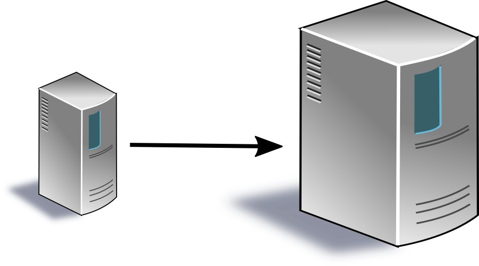
Figure 1: Scaling up improves the performance of a single machine.
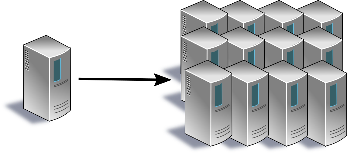
Figure 2: Scaling out distributes load over a fleet of systems.
Selection of relevant data (e.g., with a WHERE clause in SQL) is a
frequent operation, which can clearly be executed faster with
parallel processing. Note, however, that bringing lots of data to
lots of CPUs to discard most of the data is a wasteful process (in
terms of resource and energy usage), and parallelization does
nothing to improve this situation. Nevertheless, parallelization
resulting from horizontal fragmentation (also called sharding or
horizontal partitioning; to be explained in a video) is a powerful
technique, which, for example, enables scalability
- of big data processing environments such as MapReduce [DG04] and
- of NoSQL and NewSQL databases,
both of which will be covered in other sessions.
The second class of approaches could be said to prefer brain over muscle. It organizes data access differently. Indeed, we might specify, know, or learn where relevant data is located and use this knowledge to not process irrelevant data in the first place, again speeding up processing, but even with unchanged compute resources. Below, you will see sorting and the construction of index structures as examples for this class. Beyond these traditional techniques, there is considerable progress in the area of self-tuning databases (see [CN07] for a survey as of 2007 and [KAB+19] for recent work whose first author studied Information Systems in Münster). Besides, specialized hardware platforms such as Enzian offer hardware acceleration for near-memory data processing [ARC+20].
1.1. Prerequisites
- Explain binary search and the use of balanced tree structures for data access in logarithmic time.
1.2. Learning Objectives (see slides)
- Explain query processing and optimization in general
- Explain fragmentation and indexing
- Reason about typical usage scenarios
- Estimate query execution times for different query evaluation plans (after exercises)
- Explain and apply query rewriting in presence of materialized views
2. Disk based data access
Consider a typical relational database, where each relation is stored as a sequence of fixed-size blocks on disk. In case of hard disks, data is recorded on rotating magnetic platters, which cause a rotational delay before a disk’s read-write head is positioned above the correct location when a random block is to be transferred to main memory. Such a delay may be around 3ms for server disks, limiting the number of blocks that can be accessed in random order to about 300 per second. If neighboring/contiguous blocks are read from disk (e.g., for linear scans of entire relations), rotational delay occurs only once, and data can be transferred with the disk’s full bandwidth, e.g., 200 MB/s. (If you never used “bandwidth” to compute the time for the transfer of data of a given size, maybe it helps to think of velocity calculations, where you compute the time needed to cover some distance at some speed. In our setting, the size of data to be transferred corresponds to the distance to be covered, while the bandwidth corresponds to the speed…)
For solid-state drives (SSDs), no rotational delay exists, and random access of an individual block may take about 0.1ms (with 10,000 blocks per second), while high-end SSDs are able to transfer millions of 4 KiB (“Ki” is a binary prefix) blocks per second (with transfer rates beyond GB/s), see IOPS at Wikipedia if you are interested. (With SSDs, random access is still slower than sequential access because (a) each I/O request comes with overhead and (b) each random access causes a block to be read, which may be much larger than what was requested.)
3. Index structures
Index structures (or “indexes” for short; “indices” are small numbers attached to variables) are data structures that materialize data in redundant form to speed up query processing. You know indexes from everyday life. Think of a textbook, which includes a keyword index at the end. Say, you want to read about indexes in a textbook on databases. Clearly, you could read the text front to end, also learning about indexes. For faster access, you could use the keyword index and locate the index term: “index”
Next to each index term, you find pointers to pages on which the term occurs. Clearly, looking up “index” in the index and following a pointer takes some time, which defines the access latency/time which should be much lower than in front-to-back reading.
Some notes are in order. A book is broken down into numbered pages, and pages are arranged in sorted order. This corresponds quite nicely to relations, whose tuples are stored in blocks on disk; often (see Section 4 for a counter-example concerning dimension tables), those tuples are sorted according to the primary key. When the index points you to a page, say 442, you do not look at every page to find number 442 but apply a more efficient strategy, e.g., binary search; please look up binary search at Wikipedia if you cannot explain how it works. (Actually, as human beings we probably do not start in the middle but use some heuristic based on a book’s thickness.) The same is true for tuples on disk: If a tuple with a particular primary key value should be retrieved (with tuples sorted by primary key), the database management system (DBMS) can use binary search instead of a so-called sequential scan (which is reading front-to-back, scanning every tuple for matching values).
Second, the page pointers of index entries in textbooks appear in mostly random order: We do not expect index terms starting with a common prefix, say “a”, to lead to neighboring pages. Indexes, where the order of index entries does not agree with the physical order of data (here book pages) are called non-clustered or secondary indexes. Typically, non-clustered indexes contain several pointers per index term (“index structure” may be covered in different parts of the book). Different DBMSs support different index structures (various forms of trees, in particular B-trees, hash tables, bitmap indexes; please lookup B-trees at Wikipedia if you cannot explain how they are used for search in \(O(\log n)\)).
Third, books also contain other index structures, e.g., the table of contents (TOC). The TOC contains pointers from headings of chapters and sections to their starting pages. Again, if you are interested in learning about indexes, you can scan the TOC for “index.” In case of a match, you now know where to start reading (and, in contrast to the non-clustered keyword index, you can expect that “indexes” are covered thoroughly in a section if its heading contains that term). This time, the order of the index structure agrees with the order of pages, classifying the TOC as primary or clustered index: Sections that are neighbors in the TOC are also neighbors in the book itself. B-tree variants are often used for clustered indexes, e.g., to speed up tuple retrieval based on key values beyond binary search.
4. Rules of thumb
For fact and dimension tables, the following rules of thumb may serve as starting points for physical database design [GLG+08]:
- Fact table
- Implement the primary key, which consists of foreign keys to the dimension tables, as clustered index.
- Add one non-clustered index per (foreign) dimension key.
- Dimension table
- (Note: A business key is a key that has meaning in the real world or in a particular source system, e.g., ISBN for books or passport numbers for customers. For improved flexibility, so-called surrogate keys, often with strictly increasing integer values, are added in the course of ETL processing in data warehouse systems.)
- Implement the surrogate primary key as non-clustered index.
- Build a clustered index for the business key.
- Based on the workload, add additional non-clustered indexes for frequently used attributes.
5. Self-Study Tasks
The following tasks ask you to perform elementary back-of-the-envelope calculations to get a feeling for the impact of different query evaluation strategies. The videos do not cover such calculations; I hope that you can perform them anyways based on this text. Please ask if you get stuck.
Suppose that hard disks with a rotational delay of 3.3 ms and a transfer rate of 200 MB/s are used and that block transfers to main memory dominate query execution costs. Each block on disk has a size of 4 KiB and contains a number of tuples, one after the other, where the amount of storage necessary per tuple depends on the relation’s number of attributes and their data types. Typically, multiple tuples fit into a single block, and to access any of those tuples the entire block containing it needs to be loaded into main memory. All blocks belonging to one table are stored contiguously on disk.
- How long does it take to transfer a random block into main memory (based on rotational delay and transfer rate)?
- Suppose that a query of the form
SELECT * FROM Table WHERE
      Condition
is executed, whereTablecontains 8 million tuples on hard disk and has a size of 4 GiB, which is not large for data warehouse scenarios.- How long does it take to read the entire table (i.e., either
no
WHEREclause exists or it does not discard any tuple)? Tuples on disk are not sorted in any way, no index exists.
How long does it take to execute the query if
Conditionselects about 1% of all tuples? How long ifConditionselects exactly one tuple?Hint: Note that data is not sorted. You may want to think about best, worst, and average cases. For the case of “about 1% of all tuples”, at what point in time can the query executor be sure to have seen all matching tuples?
Suppose that
Conditionhas the formAttribute = Valueand thatTableis sorted byAttribute.How long does it take to execute the query using binary search if
Conditionselects 1% of all tuples? How long ifConditionselects exactly one tuple?
- How long does it take to read the entire table (i.e., either
no
- Watch the videos provided in Learnweb. Ask any questions that
you may have.
The second video ends with a question concerning the guarantees of query optimization (slide 9): Why does optimization not lead to the selection of the plan with lowest cost?
The answer to that question rests upon the use of heuristics for query optimization.
To train relational algebra, the data for the optimization example of the fourth video is accessible as Gist for RelaX (you may have used RelaX for self-study tasks related to the Relational Model).
pi B, D ( sigma A = 'c' and E = 2 and R.C = S.C (R x S))
- The video on materialized views contains a question at 9:10, which we will discuss in class. You may find that the subsequent part hints at an answer.
(Again, some thoughts are available separately.)
6. Tentative Session Plan
- Questions on previous topics
- Interactive review of self-study tasks
- For the sample materialized view and queries contained in the slides: Discuss how the view can be used to speed up the queries.
- Task 3 of Exercise Sheet 2.
- If time permits, we may look at real query evaluation plans.
(With PostgreSQL, type
EXPLAINin front of a SQL query to see its plan; useEXPLAIN ANALYZEto also execute it. Make sure that DBMS statistics are current first, e.g., withVACUUM ANALYZE.) - Introduction to next topic
Bibliography
- [ARC+20] Alonso, Roscoe, Cock, Ewaida, Kara, Korolija, Sidler & Wang, Tackling Hardware/Software co-design from a database perspective, in: CIDR 2020, 10th Conference on Innovative Data Systems Research, 2020. http://cidrdb.org/cidr2020/papers/p30-alonso-cidr20.pdf
- [CN07] Chaudhuri & Narasayya, Self-Tuning Database Systems: A Decade of Progress, in: Proceedings of the 33rd International Conference on Very Large Data Bases (VLDB), 2007. http://www.vldb.org/conf/2007/papers/special/p3-chaudhuri.pdf
- [DG04] Dean & Ghemawat, MapReduce: Simplified data processing on large clusters, in: 6th Symposium on Operating Systems Design and Implementation, 2004. https://static.usenix.org/publications/library/proceedings/osdi04/tech/full_papers/dean/dean.pdf
- [GLG+08] Galindo-Legaria, Grabs, Gukal, Herbert, Surna, Wang, Yu, Zabback & Zhang, Optimizing Star Join Queries for Data Warehousing in Microsoft SQL Server, in: 24th International Conference on Data Engineering, 2008.
- [KAB+19] Kraska, Alizadeh, Beutel, Chi, Kristo, Leclerc, Madden, Mao & Nathan, SageDB: A Learned Database System, in: CIDR 2019, 9th Biennial Conference on Innovative Data Systems Research, 2019. http://cidrdb.org/cidr2019/papers/p117-kraska-cidr19.pdf
License Information
Source files are available on GitLab (check out embedded submodules) under free licenses. Icons of custom controls are by @fontawesome, released under CC BY 4.0.
Except where otherwise noted, the work “OLAP Optimization”, © 2018-2022 Jens Lechtenbörger, is published under the Creative Commons license CC BY-SA 4.0.
Created: 2025-09-30 Tue 12:48