OLAP and ETL
1. Context
In previous classes you have seen multidimensional models to support
OLAP (online analytical processing). Here, we start from the
observation that dimension hierarchies can be formalized naturally
in terms of relational schemata (Section 2.1),
which is important for proper formulation of GROUP BY queries in
SQL and which will be used in a subsequent session for data
warehouse schema design. Afterwards, we contrast OLTP (online
transaction processing) with OLAP. We discuss the need for ETL
(extract, transform, load) processes (Section 3),
briefly recalling star and snowflake schemata (Section
3.1) and introducing the concept of data lakes
(Section 3.2).
Finally, we present SQL extensions for OLAP (Section 4).
Besides, some thoughts on self-study tasks are available
separately.
1.1. Prerequisites
Please refresh your SQL skills if necessary, in particular with
aggregation using GROUP BY and HAVING. Maybe solve the
following two tasks and please do not hesitate to ask (on- or
offline).
Over the schema of database benchmark TPC-H, express a query that selects order volume (as sum over totalprice) and contact information (name, address, name of nation, and phone) for customers in region EUROPE whose order volume exceeds 1,000,000.
In Learnweb, you find scripts to set up the TPC-H schema in a PostgreSQL database for your own experiments (with these instructions as suggested previously).
Consider the following queries:
SELECT a, b, SUM(c) FROM ... WHERE ... GROUP BY a, bSELECT a, SUM(c) FROM ... WHERE ... GROUP BY a
Suppose that the FD a \(\to\) b holds. What can you say about the relationship between results for both queries in terms of the number of rows and aggregate values?
1.2. Learning Objectives
- Contrast OLTP and OLAP
- Formulate SQL queries with OLAP extensions in view of dimension hierarchies and functional dependencies
- Discuss necessity of ETL processing
- Explain the term Data Lake
2. Multidimensional Schemata
Multidimensional schemata are used to model data warehouse scenarios at a conceptual level (after requirements specification and prior to logical implementation and physical optimization). At their core, such models specify the multidimensional structure of events, e.g., calls, sales, repairs, deliveries, medical diagnoses. For sales, the multidimensional structure might include information related to time, place, customer, product, each of which is specified by a dimension schema as defined subsequently. Moreover, each event is described by number of numerical values, called measures, e.g., price, volume, profit.
2.1. Dimension Schemata
A dimension schema can be perceived as special form of relation schema: Dimension schemata contain attributes, which are called dimension levels. Also, every dimension schema is associated with inter-relational integrity constraints, which are visually represented in terms of a dimension hierarchy, relating (instances of) some dimension levels to others.
Consider the multidimensional schema of Figure 1, for which a slightly different representation was shown in an earlier lecture. (In this figure, we introduce an additional box to represent each dimension schema, which is then connected to its most detailed dimension level. The most detailed level is frequently some form of identifier, indicated by “ID” as part of level names.) That model embeds multiple dimension schemata, namely schemata about time, customers, garages, vehicles. The schema for garages contains dimension levels GID, GeogrRegion, Country, and GarageType. Recall that arrows between dimension levels represent many-to-one relationships, e.g., many garages belong to each region, while each garage is located in exactly one region.
Notice that many-to-one relationships and functional dependencies express the same constraint: Attribute GID functionally determines GeogrRegion.
The importance of this observation is that it opens the door to standard relational database design methods in the domain of multidimensional data warehouse design. In a subsequent session, you will see how 3NF normalization with synthesis carries over to multidimensional design.
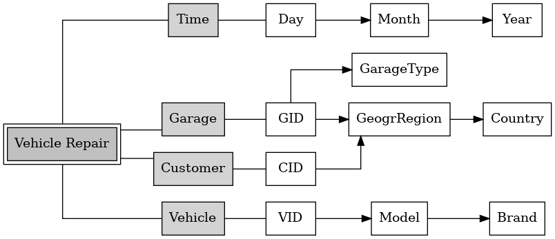
Figure 1: Multidimensional schema based on Fig. 7 of [SBHD99].
2.1.1. Self-study tasks
- Convince yourself that many-to-one relationships and functional dependencies embody the same type of constraint.
- Consider level Day in the Time dimension of Figure 1. What attribute in Task 1 of Exercise Sheet 2 corresponds to level Day?
3. OLTP, OLAP, Hybrids, and Integration
OnLine Transaction Processing (OLTP) refers to the tracking of events in support of business processes (e.g., placement of an order, initiation of a shipment, a payment) by means of database transactions in so-called operational databases. With OLTP, transactions are usually short and refer to individual (or few) tuples (insertions, updates, and so-called point-queries that target individual tuples, e.g., a query for the details of the order with ID 42). The efficient execution of such transactions is usually supported with index structures, a topic which will be revisited in a later session on OLAP optimization.
In contrast, OnLine Analytical Processing (OLAP, coined by Codd et al. [CCS93]) refers to the analysis of large amounts of data, usually with complex aggregation queries in a read-only manner. Essential aspects of OLAP are covered by the acronym FASMI (Fast Analysis of Shared Multidimensional Information, see [PC95]), which emphasizes the expected speed of query processing for analysis purposes and the multidimensional nature of data that is typical for data warehouse systems.
As argued by Plattner [Pla14], OLTP and OLAP are not that different in the real world: Also for OLTP, 80% of the workload consists of read accesses, while “less than 10% of the actual workload are queries that modify existing data, e.g., updates and deletes.” The major difference lies in the selectivity of queries. While usually only few tuples are accessed per query with OLTP, large amounts are accessed and usually aggregated with OLAP.
With the advent of powerful in-memory database systems, several hybrid systems arose, which promise high performance for OLTP and OLAP workloads in a single system or based on a coupling of systems, in particular of databases and big data systems. Such hybrid systems may be branded as OLTAP, OLXP, or HTAP, see [OTT17] for a survey and challenges if you are interested.
A company may need to obtain an integrated view over several operational databases for company-wide OLAP and other types of analytics (potentially involving deep/machine learning). Indeed, according to a frequently cited definition by Inmon (which you saw earlier), “integrated” is a key characteristic of data warehouse systems ([CD97] attributes this definition to Inmon in 1992). For integration purposes, ETL processing can extract relevant data from operational databases (and other data sources), transform data originating in separate systems (each of which might come with different scope, modelling choices, data types, formats, conventions) into an integrated target schema, and load it into a separate database, the data warehouse. Then, OLAP happens on top of this data warehouse, which can be optimized for OLAP access patterns (instead of OLTP access patterns), which we will revisit in a separate session.
For ETL processing, numerous software tools exist, which support the graphical or programmatic specification, execution, and monitoring of ETL processes. To get an idea how such tools look like, you could watch some tutorials for Pentaho Data Integration, a free/libre and open source ETL tool.
Note that different combinations of the letters “T” and “L” are possible. With ELTL, extracted data may be loaded into a separate system first before being transformed and loaded into a data warehouse. Two prominent examples for such initial loading are provided by data vaults and data lakes, to be revisited subsequently.
With ELT, data may be loaded into the (powerful) target system, where it is transformed (either virtually during query processing or in materialized form in separate tables). With EL, data is loaded elsewhere without transformation (e.g., into a data lake). Also, while “traditional” ETL supposes a one-way road from source databases to target data warehouse via periodic (e.g., per day or per week) batch processing, the scope of ETL processing has broadened to bi-directional data flows [DCS+09] (data sources may benefit from data cleaning as part of ETL, and analysis results may be used in daily business processes) between different types of data processing systems (not only data “living” in databases but also streams arising from sensors or APIs and interactions on the Web).
3.1. Stars and Snowflakes
You have already seen that conceptual data warehouse schemata can be implemented in different logical (relational) variants, the two most famous ones being the star schema and the snowflake schema. In a nutshell, a snowflake schema is a 3NF implementation of a multidimensional scenario, while a star schema only contains one (usually denormalized) table per dimension.
An ETL process might then populate the chosen form of schema.
Beyond learning objectives, real-world projects might design their ETL processes based on data vault modeling, which is a relational (logical) modeling approach for data warehousing proposed and explained by Dan Linstedt. It can be perceived as alternative to—or preparatory integration step for—star or snowflake schema modeling. In a nutshell, a data vault represents timestamped raw data. The paper [GGH+19] discusses the use of data vault modeling in connection with data lakes from a research perspective.
3.2. Data Lake
According to the overview [SD21], a “data lake is a scalable storage and analysis system for data of any type, retained in their native format and used mainly by data specialists (statisticians, data scientists or analysts) for knowledge extraction.” Data lakes may contain structured, semi-structured, and unstructured data, where no schema is defined ahead of time. Instead, raw data is available for arbitrary future analyses, offering a high degree of flexibility and use-case independence, but potentially coming with data quality issues and integration overhead before analysis. This approach is also called schema-on-read, to be contrasted with schema-on-write, which is inherent to data warehouses where only data adhering to a strict schema is available.
While the term “data lake” was initially tied to an implementation based on Hadoop with its distributed file system (HDFS), nowadays various ecosystems are in use (e.g., distributed file systems, NoSQL stores—to be revisited in a subsequent session, cloud object stores, messaging systems) [SD21]. In our context, a data lake may serve as just another data source to be integrated into a data warehouse. Several architectural patterns combining data lakes and data warehouses are discussed in [Her20] (e.g., a sequential approach, where the data lake serves as integration layer and forms the only source for the data warehouse, a parallel approach where data lake and data warehouse exist as isolated systems, and approaches with different degrees of integration, e.g., to make analysis results obtained on top of the data warehouse available in the data lake and vice versa). In other sessions, you will see techniques such as MapReduce and Spark that can be applied for analyses on top of data lakes.
As one pointer for recent research and development regarding data lakes, we point out the notion of delta lakes, which provide ACID transactions over cloud object stores [ADS+20], thereby promising to overcome consistency challenges of data lakes. The authors call this the “lakehouse” paradigm “that combines the key features of data warehouses and data lakes: standard DBMS management functions usable directly against low-cost object stores.” Code is available as free/libre and open source software.
3.3. Self-study tasks
- Read Chapter 3 in [Pla14] (available in Learnweb) by Prof. Hasso Plattner, a co-founder of SAP, and answer this question: What does the author think about ETL processing and why?
Given your knowledge about data warehousing, why might it be difficult or impossible to abandon ETL processing entirely (despite Prof. Plattner’s arguments)?
You might read the Introduction and the Conclusions of [YRX+20] (accessible from university network) for arguments. (The remainder of the paper is not less interesting. See for yourself.)
4. OLAP in SQL
The SQL standard includes extensions of the GROUP BY clause, which are
useful for OLAP applications (some extensions were added to SQL:1999 and
revised in SQL:2003, but are still not supported in all DBMSs), in
particular GROUP BY CUBE and GROUP BY ROLLAP, whose ideas originate
in the seminal paper [GCB+97].
In SQL, each of the keywords GROUP BY CUBE and GROUP BY ROLLUP is
followed by a list of attributes. With GROUP BY CUBE (A1, A2, ...,
An), aggregation is performed for every sub-list of (A1, …,
An) and the results of all these aggregations are combined into an
overall query result. (Note that a list with \(n\) elements has \(2^n\)
sub-lists. So, such a query is best understand as simultaneous
computation of lots of traditional GROUP BY queries.)
With GROUP BY ROLLUP (A1, A2, ..., An), aggregation is performed for
every prefix of (A1, …, An). (A prefix of list \((A_1, \ldots,
A_n)\) is a sub-list \((A_1, \ldots, A_k)\) for some \(k \leq n\). For
\(k=0\) the empty list arises, for \(k=n\) the entire list.
E.g., GROUP BY ROLLUP (A, B, C) leads to aggregations
- grouped by
A, B, C, - grouped by
A, B, - grouped by
A, and - without group by (computing the so-called grand total).
These extensions of GROUP BY (and further additions of SQL:2003) are
explained with slides and video recordings for some of those slides
from a past lecture in Learnweb. Work through the slides, maybe watch
the videos.
4.1. Self-study
Consider a ROLLUP query such as the following one (also contained
in slides and video in Learnweb).
SELECT supplier, s_nationkey, n_regionkey, sum(sales)
FROM transaction, supplier, nation
WHERE supplier = s_suppkey and s_nationkey = n_nationkey
GROUP BY ROLLUP (n_regionkey, s_nationkey, supplier)
Make sure that you understand this query. In
particular, what happens if the order of group-by attributes is
reversed, i.e., we have GROUP BY ROLLUP (supplier, s_nationkey, n_regionkey)?
What happens if for a clause such as
GROUP BY ROLLUP (supplier, part, customer)?
(If you are not sure, please try this out.)
5. Tentative Session Plan
- Interactive review of self-study tasks
- Recall the differences between star and snowflake schemata. How would
the dimension for
garagebe implemented under each variant? - For a star schema, create a sample relation for dimension
garageof Figure 1 with at least two different countries, two regions per country, two garages per region, two types of garages, and two garages per type. Observe the many-to-one relationships specified by the arrows while doing so. Afterwards, analyze the functional dependencies (FDs) among pairs of attributes. Which ones do you find, which ones do you expect to be satisfied in every instance? What about keys? - First look at Task 2 of Exercise Sheet 2
- Introduction to next topic
Bibliography
- [ADS+20] Armbrust, Das, Sun, Yavuz, Zhu, Murthy, Torres, van Hovell, Ionescu, Łuszczak, Świtakowski, Szafrański, Li, Ueshin, Mokhtar, Boncz, Ghodsi, Paranjpye, Senster, Xin & Zaharia, Delta Lake: High-Performance ACID Table Storage over Cloud Object Stores, Proc. VLDB Endow. 13(12), 3411-3424 (2020). https://doi.org/10.14778/3415478.3415560
- [CCS93] Codd, Codd & Salley, Providing OLAP (On-line Analytical Processing) to User-Analysts: An IT Mandate, Arbor Software, (1993). https://web.archive.org/web/19970612201539/http://www.arborsoft.com/essbase/wht_ppr/coddTOC.html
- [CD97] Chaudhuri & Dayal, An Overview of Data Warehousing and OLAP Technology, SIGMOD Rec. 26(1), 65-74 (1997). https://doi.org/10.1145/248603.248616
- [DCS+09] Dayal, Castellanos, Simitsis & Wilkinson, Data integration flows for business intelligence, in: Proceedings of the 12th International Conference on Extending Database Technology: Advances in Database Technology, 2009.
- [GCB+97] Gray, Chaudhuri, Bosworth, Layman, Reichart, Venkatrao, Pellow & Pirahesh, Data Cube: A Relational Aggregation Operator Generalizing Group-By, Cross-Tab, and Sub-Totals, Data Min. Knowl. Discov. 1(1), 29-53 (1997). https://doi.org/10.1023/A:1009726021843
- [GGH+19] Giebler, Gröger, Hoos, Schwarz & Mitschang, Modeling data lakes with data vault: practical experiences, assessment, and lessons learned, in: International Conference on Conceptual Modeling, 2019. https://doi.org/10.1007/978-3-030-33223-5_7
- [Her20] Herden, Architectural Patterns for Integrating Data Lakes into Data Warehouse Architectures, in: International Conference on Big Data Analytics, 2020. https://doi.org/10.1007/978-3-030-66665-1_2
- [OTT17] Özcan, Tian & Tözün, Hybrid Transactional/Analytical Processing: A Survey, in: Proceedings of the 2017 ACM International Conference on Management of Data, 2017. https://doi.org/10.1145/3035918.3054784
- [PC95] Pendse & Creeth, What is OLAP?, The OLAP Report, (1995). https://web.archive.org/web/19970330110156/http://www.olapreport.com/fasmi.htm
- [Pla14] Plattner, A Course in In-Memory Data Management: The Inner Mechanics of In-Memory Databases, Springer-Verlag, Berlin, Heidelberg, 2014.
- [SBHD99] Sapia, Blaschka, Höfling & Dinter, Extending the E/R Model for the Multidimensional Paradigm, in: Advances in Database Technologies. ER 1998. LNCS 1552, 1999. https://doi.org/10.1007/978-3-540-49121-7_9
- [SD21] Sawadogo & Darmont, On data lake architectures and metadata management, Journal of Intelligent Information Systems 56(1), 97-120 (2021). https://doi.org/10.1007/s10844-020-00608-7
- [YRX+20] Yang, Rae, Xu, Shute, Yuan, Lau, Zeng, Zhao, Ma, Chen, Gao, Dong, Zhou, Wood, Graefe, Naughton & Cieslewicz, F1 Lightning: HTAP as a Service, Proc. VLDB Endow. 13(12), 3313-3325 (2020). https://doi.org/10.14778/3415478.3415553
License Information
Source files are available on GitLab (check out embedded submodules) under free licenses. Icons of custom controls are by @fontawesome, released under CC BY 4.0.
Except where otherwise noted, the work “OLAP and ETL”, © 2019-2022 Jens Lechtenbörger, is published under the Creative Commons license CC BY-SA 4.0.
Created: 2025-09-30 Tue 12:48